Intended for software and data engineers with an interest in database internals, this content explores the unusual challenges and solutions involved in diffing across different SQL databases.
Table of Contents
- Introduction
- Part 1 - Calculating hashes
- Part 2 - Splitting tables
- Part 3 - Implementing the diff
- Conclusion
Introduction
In the world of data engineering, diffing datasets - that is, pinpointing all the differences between two tables - is potentially a very useful operation. For example, it can be used for validating data migrations, data versioning (think git), detecting data corruption, gradual backups, auditing, and the list goes on. At its core, diffing tables should be straightforward: Just match the rows by their primary key, and then go row-by-row and compare the values. But when the diff has to work on tables that belong to different databases, and reside on different servers, things get a little trickier, as we will soon see.
In 2022, a client approached me to do just that - create an open-source tool that could efficiently diff large SQL datasets across different databases and servers. We wanted to create the best tool that we could, and for that, we needed to support all major SQL databases, and have the tool deliver significant performance improvements over conventional approaches. As the project progressed, a few substantial challenges became very apparent, although only by the end of the project, we came to realize their full magnitude and scope.
Networking, commonly enough, was the first challenge we faced. Transferring data over the network can be slow and costly. Because the databases might reside on different servers, comparing the data directly would involve downloading huge tables, which we wanted to avoid. Another issue is that many databases enforce query time-outs that terminate long-running queries. That makes sense, except that even a simple COUNT(*) can time-out on very large tables, if the time-out configuration is strict. So we needed to make sure to query a limited number of rows each time. And, there's also lag to deal with. Our solution needed to be robust enough to handle real-world situations, without prior knowledge about the network, the server, or their configurations.
The second challenge is that every SQL database has its own standards and peculiarities. Programmers that want to support a large number of databases have to stick to common SQL operations, or try to bridge the gap themselves if no such operation exists (like a polyfill). Even when an operation is supported by all the databases, each one behaves differently, or has a different syntax. This is also true for basic operations, like the SUM() function, NULL comparisons, for creating substrings, casting between types, and so on. ORMs aren't helpful in this situation, because they don't provide many of the functions and features that we need. We had to write our own infrastructure.
The third challenge is that SQL databases were designed from the point-of-view of data retrieval and business logic. They were not designed for running algorithms or complicated calculations. Many of the operations and constructs that we take for granted in procedural or functional programming, like loops, arrays, or memory, are not available in standard SQL. A few databases do offer these as extra features, but that isn't something we could rely on, if we wanted wide support.
Despite these challenges, we were able to thread the needle and create a capable and efficient diffing tool, and by the end of this article, you will know how to make one too.
Before we get into the implementation details, let's take a look at the algorithm that we will be using.
The algorithm in a nutshell: Divide, Hash, And Conquer
We started with a simple insight: we don't need to download data if it's equal. Instead, we can compare hashes of the data, like a checksum, to detect the differences. When the checksums differ, we can drill-down using a divide-and-conquer algorithm, eventually zoning in on the rows that are different. The basic process is very simple: Hash the two tables. If they are different, split them both into smaller segments, and repeat the process for each pair of segments. When the segments are small enough, if they are different, download and compare them directly. That way, two identical tables will only require a single hash pass to validate, and tables with few differences will only require a few small segments to be downloaded and compared directly. Since our use-case was mainly validation and gradual updates, we could make the assumption that most of the data would be the same.
Here is the algorithm:
- Split both tables into corresponding segments based on their primary keys
- Calculate a hash checksum for each segment pair
- Compare the hashes:
- If the hashes match → Great! Those segments are identical (no need to download any rows)
- If the hashes differ → We have two options:
- For small segments: Download both segments and compare them in memory
- For large segments: Recursively split them into smaller pieces and repeat the process
This algorithm, while simple, can't be written entirely in SQL, of course. We chose Python as the main language of the tool, because of its wide-support and ease of use. Python sometimes gets criticized for its speed, but in this case, all of the performance bottlenecks were in the database queries, and not in Python.
Not so simple
However, putting a simple idea into practice isn't always straightforward. For one thing, in order to calculate a stable hash, we have to ensure a text-perfect synchrony between the two databases. Small formatting issues can cause the hashes to differ, even if the data is the same. And then there are timezones, and different precisions. Secondly, splitting the table into even segments ended up being much more difficult than expected, due to limitations in SQL (hint: we can't use OFFSET). As the reader will soon see, we faced a long list of unexpected obstacles and challenges, both big and small.
The following text is a technical exploration of the main obstacles that we encountered on our way to a cross-database highly-efficient diff, and how we overcame them, sometimes with an elegant insight, and sometimes with hard meticulous work. It was a long journey full of hidden complexities and surprising solutions, and it ended up challenging a lot of my assumptions about how databases work under the hood, what they can and can't do, and about what is the best way to interface with them programmatically. I hope the reader will find it interesting, or at the very least, amusing.
This text assumes some familiarity with SQL and general programming concepts. I will try to provide context and explanations for key concepts to ensure readers of all levels can follow along.
Part 1 - Calculating hashes
The first step of our diffing algorithm is to calculate hashes for each block of data. If the corresponding blocks of data have the same hash, we can avoid having to download the data unnecessarily. For that to work reliably enough, we need a robust hashing algorithm, that can run on every database we plan to support, and that is fast enough to not become a bottleneck. We soon found out calculating a hash in SQL is no walk in the park, especially because we need to support different databases, each with their own idea of how to represent values.
Good old MD5 to the rescue
MD5 is a popular and well-rounded hash function. It is also the only hashing function that is supported on every database on our list. While MD5 was abandoned as a cryptographic algorithm many years ago, it's still useful in non-adversarial situations. It is fast and has a very low collision rate for our use case.
Unfortunately, soon we discovered that one of the databases we planned to support, namely SQL Server, has a very slow MD5 function. In fact it is around 100 times slower than the PostgreSQL MD5 function! After some experimentation, we decided it would be impractical to use it, and dropped support for SQL Server. It's the only database for which we ended up dropping support. It was a difficult decision, but we couldn't find an acceptable workaround.
Sums can overflow
The MD5 function in SQL only accepts columnar data, and cannot compute several rows at once. That leaves us with the responsibility to add up the MD5 values produced for each row. On different databases, some MD5() functions return a string, while others return a number. We had to normalize all the return values into an integer, so we can sum them up.
Unfortunately, in many databases SUM() can overflow, which happens when it passes its maximal value (yes, even with bigint and decimal). By itself, an overflow into a negative number wouldn't interfere with the hash function, but only some databases do so. Many databases throw an error instead, or return NULL. When that happens, we have no way to access the result, and the computation is wasted. Our solution was to cut the MD5 values into smaller numbers, and also limit how many rows we sum per batch, to prevent an overflow at all costs.
Through experimental tests, we landed on taking only the lower 60 bits of the MD5 hash. In retrospect, this is the one choice we made that I have my doubts about. With 60 bits, the chance of collision (i.e. having two different values that yield the same hash) is vanishingly low for our use case, but it's still much higher than what we would get with a full MD5 value, and the risk of collision gets even worse because we are comparing only the sums of the hashes, and not the hashes themselves. Limiting the summed up batches to 16K rows helps keep the risk of collision low. Still, I wonder if it wouldn't have been better to use a bigger number (i.e. more bits), and query smaller batches, even at the expense of some speed.
For situations when a miss could be catastrophic, it might be worth considering a simpler alternative algorithm, in which we only split the table once, and then download all the hashes. It will be much slower, but mathematically, it will be much safer.
In our implementation we tried to make it easy to raise the number of bits, using a small change to the source code. For example, here are the MySQL & PostgreSQL expressions to generate an MD5 and take the lower 60 bits (rewritten as templated SQL):
MD5_HEXDIGITS = 32
CHECKSUM_HEXDIGITS = 15		# We take the lower 60 bits
MD5_OFFSET = 1 + MD5_HEXDIGITS - CHECKSUM_HEXDIGITS


-- MySQL: md5_to_int(s) =
cast(conv(substring(md5({s}), {MD5_OFFSET}), 16, 10) as unsigned)

-- PostgreSQL: md5_to_int(s) =
('x' || substring(md5({s}), {MD5_OFFSET}))::bit({CHECKSUM_HEXDIGITS*4})::bigint
For those interested in the Python source code that generates these queries, you can find these functions here and here. Note that these links lead to sqeleton, which is the SQL library powering Reladiff.
Column values need to be normalized
MD5 functions run on strings, and for their result to be consistent, the input strings need to be consistent as well. This means that the same value must always be represented by the same string, on every database. While text columns are usually consistent between databases, other types are not. We had to pay special attention to the following types.
Booleans
This one at least was straightforward. Some databases use zeros and ones, while others use "True" and "False", and others "T" and "F". We just convert them all to a number, which forces them into 0 or 1.
Numbers & Precision
This one was anything but straightforward. In each database, the functions for displaying values are different. They have different names, different parameters, and different behaviors. But that was the least of our worries.
The main difficulty in normalizing numbers was to format them with the right precision. Each database has a different limit on precision for its numbers and dates. Precision essentially means how many digits after the decimal point are stored in the databases. For example, Snowflake supports 9 digits after the dot, while Presto supports 3. Most databases support 5 or 6. In addition to the maximum precision each database is capable of, each column may have its own user-defined precision settings, which are stored as part of the schema. That means that while Snowflake supports 9 digits, a specific float column in Snowflake might allow only 4 digits after the dot, or 2, etc.
Why is that a problem? Let's say we copied some data from Snowflake to MySQL. As a result, floats that had 9 digits after the dot in Snowflake will be truncated to 6 digits in MySQL! As we turn both into a string argument for the MD5 function, we will get different results, even though, from our perspective, the data is supposed to be equal. On the other hand, we do want to compare to the highest precision that makes sense, so we don't miss subtle changes in the data. To solve it, we check the precision settings of each column, by querying the schema, and then, per column, negotiate the highest supported precision between both columns (one from each database). We then use that negotiated precision to round the value when converting it to a string.
There were a few more small obstacles. For example, sometimes we needed to use different code between precision==0 vs. precision>0, and some databases insisted on annotating big numbers with commas, such as Databricks.
Here, for example, is the code for number normalization with databricks:
def normalize_number(self, value: str, coltype: NumericType) -> str:
    value = f"cast({value} as decimal(38, {coltype.precision}))"
    if coltype.precision > 0:
        value = f"format_number({value}, {coltype.precision})"
    return f"replace({self.to_string(value)}, ',', '')"
Normalizing timestamps
Having already dealt with numbers, I thought this would be easy. How much harder can it be to normalize timestamps, compared to regular numbers? Well, it ended up being one of the most challenging tasks of the project.
Timestamps, like numbers, support varying precision. But unlike with numbers, when rounding a timestamp to a lower precision, some databases will always floor it (i.e. always round it down), while others round it to the nearest value. For example, let's say we have a timestamp in Snowflake that ends with 1.999999999, and we copy it to a PostgreSQL database. That timestamp will get stored rounded up to 2 by PostgreSQL, which means we should also round it up on Snowflake's side, before comparing them. But if instead we copied the timestamp to DuckDB, it would round it down to 1.999999, and we would need to round it down on Snowflake when diffing them. We ended up having to implement both round-down and round-up versions for each database, and decide which one to use according to which column had the lowest precision. Each function can end up quite complicated.
Additionally, timestamps may have timezones (and they may not). To fix the timezone issues, we set the timezone of the session to UTC. That, of course, is a different command in each database. Then we format the timestamp as well as we can (not all databases have adequate formatting functions), and then do a bit of database-specific text editing to make them conform to the canonical format. The format we chose is YYYY-MM-DD HH:mm:SS.FFFFFF , a fairly standard representation, that in most databases doesn't take too much code to produce. However, in many cases, the code to produce a rounded-down version of the date, ends up looking very different from the code to produce a rounded-up version.
Example code for PostgreSQL (see in github):
def normalize_timestamp(self, value: str, coltype: TemporalType) -> str:
    if coltype.rounds:
        return f"to_char({value}::timestamp({coltype.precision}), 'YYYY-mm-dd HH24:MI:SS.US')"
    timestamp6 = f"to_char({value}::timestamp(6), 'YYYY-mm-dd HH24:MI:SS.US')"
    return (
        f"RPAD(LEFT({timestamp6}, {TIMESTAMP_PRECISION_POS+coltype.precision}), {TIMESTAMP_PRECISION_POS+6}, '0')"
    )
Example code for DuckDB (see in github):
def normalize_timestamp(self, value: str, coltype: TemporalType) -> str:
    # It's precision 6 by default. If precision is less than 6, we remove the trailing numbers.
    if coltype.rounds and coltype.precision > 0:
        return f"CONCAT(SUBSTRING(STRFTIME({value}::TIMESTAMP, '%Y-%m-%d %H:%M:%S.'),1,23), LPAD(((ROUND(strftime({value}::timestamp, '%f')::DECIMAL(15,7)/100000,{coltype.precision-1})*100000)::INT)::VARCHAR,6,'0'))"

    return f"rpad(substring(strftime({value}::timestamp, '%Y-%m-%d %H:%M:%S.%f'),1,{TIMESTAMP_PRECISION_POS+coltype.precision}),26,'0')"
Part 2 - Splitting tables
So far, we chose a hash function, made sure we can aggregate it, and normalized the data. After this long and arduous process, we have a hash function that is stable and consistent across all databases! Now we get to the next step, no less challenging: splitting the table into smaller chunks.
Table-splitting is a fundamental operation in Reladiff, which we employ for three separate reasons. The first reason is baked-in as a requirement of our diffing algorithm: divide-and-conquer requires that we divide. The second reason is parallelization: By splitting tables into smaller chunks, we can process them in parallel, and get the results back much quicker. The third reason is that we need to limit how many rows we query at one time, partly because SUM() could overflow, but mainly because if a query runs for too long, it could time-out. When we tested our initial attempts on large tables, the hash calculations would often time-out. On very large tables, even COUNT() would sometimes time-out. It became clear that splitting the tables into smaller, more digestible segments, should be the first step of our diffing algorithm, even when the divide-and-conquer isn't needed.
If you're experienced with SQL, take a minute to think. How would you split a table?
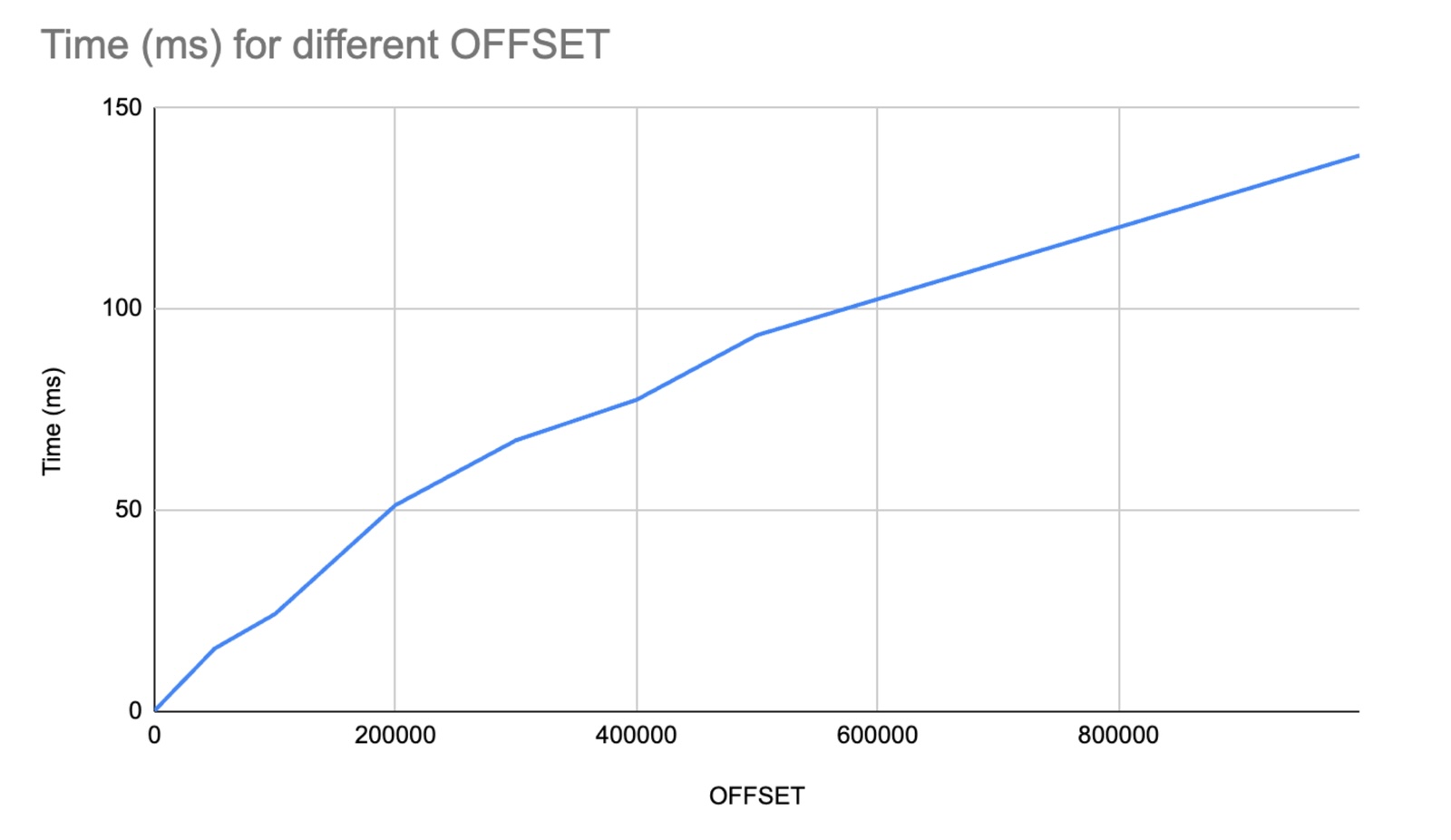
Offsetting expectations
In procedural languages, arrays are easy to slice, with a bit of pointer arithmetic that runs in constant time. In SQL databases, OFFSET is an O(n) operation! That is, the run-time of OFFSET depends on the size of the offset, and high values produce a notable effect on the running time of the query. This might seem counter-intuitive to those with a procedural-language background, but there's a rationale: the offset of each row depends entirely on the query's order, filters, and joins. It can also change whenever a new row is inserted. So while caching the offsets is theoretically possible, it is understandable why databases would not prioritize it as a feature. It's also often fine as it is for analysts or old-school websites, that usually only need to show the first few pages to whoever is querying. But this limitation disqualifies OFFSET from being useful for full-table pagination, if performance is of any concern. If we tried to split the table m times, we'd end up with O(n*m) operations. Similarly, counting inside a window function is an O(n) operation, and filtering on the counter won't prevent the filtered rows from being read into memory and slowing down the query.
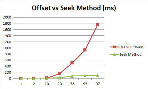
Keyset pagination
So how do modern websites implement pagination? They use a technique called keyset pagination, sometimes called seek pagination, which uses the values of a unique indexed column to determine the starting point for each page. This is usually done by choosing an ID column or a timestamp, and then using the value of that column in the last row of the previous page as the starting point for the next page. For keyset pagination to work, we need two things: Firstly, the query needs to be ordered by the keyset column. Secondly, the column has to be indexed, so that filtering on it won't trigger a full-table scan.
Example query for keyset pagination:
SELECT * FROM table WHERE id >= {lastId} LIMIT {pageSize} ORDER BY id;If you're interested in more detail, this article and the first part of this article go deeper into keyset pagination, and other kinds of pagination.
Keyset pagination is great for reading the pages one by one. But for our purposes, we wanted something better, that would allow us to read the pages in parallel.
Keyset segmentation
Keyset pagination is suitable when reading the pages one by one. In each response, we can read the last value, and use it in the next request. But for Reladiff, we wanted to query the pages in parallel, which meant we wanted to be able to get multiple pages at once, and fast. To do that, we needed to know the values that anchor the pages, before actually reading the pages themselves. The solution we chose was to get the min() and max() values of the keyset column, assume a uniform distribution, and split the column-space into the desired number of segments. For example, if our table had an ID column with values between 1000 and 2000, and we wanted 2 segments, we would split the range into 1000-1500 and 1500-2000. Note that the segmenting value, in this case 1500, doesn't have to actually exist in the table. The segmentation will work either way, since all it does is constrain the space of values. Similarly, the column doesn't have to be unique, we just have to take into consideration that having many duplicate values will lead to bigger pages, since all equal values will return in the same page. (unless there is a secondary pagination mechanism, but let's not get into that)
Example query for keyset segmentation:
SELECT * FROM table
WHERE id >= {pageStart} AND id < {pageEnd}
ORDER BY id
The performance profile of keyset segmentation is the same as keyset pagination, except that segmentation allows us to process the segments in parallel. While keyset segmentation is a clear win in terms of performance, there are also downsides: For one thing, we can't guarantee the exact size of the page we are reading. And another: On some databases, like Snowflake, the initial call to min()/max() isn't cached in the index, adds a small delay.
However, our task involves segmenting two tables, often in different databases, requiring their segments to match precisely. This adds its own costs in the form of additional complexity, as we'll see below.
Value distribution
It makes sense to assume that a primary key would have a uniform distribution, more or less. And in fact, that is usually the case, since most tables have an auto-increment column, in the form of an integer ID. However, there are plenty of tables for which this isn't true. In fact, primary keys can take many forms. They can be a UUID, and they can be an alphanumeric string. They might be split over multiple columns (i.e. compound keys), and they might contain big gaps in their values, left behind by deleted data. In short, non-uniform distributions are always possible, and they lead to dividing the key space unequally. It means that some pages can turn out to be huge, while others very small, or even empty, and that can affect the performance of the tool. While a real concern, most real-world key distributions are uniform enough to divide and conquer. In our tests, even very non-uniform tables were still processed in an acceptable amount of time. Nonetheless, that is a limitation to keep in mind.
So far I can think of two solutions to this problem. The first is sampling the segment to estimate the distribution of the key, an O(n) operation, but one that is fairly safe to cache. A simpler approach might be to dynamically update the bisection parameters, if too much recursion is detected. But these two are theoretical so far, and haven't been tried.
Alphanumerics & UUIDs
UUIDs (Universally Unique Identifiers) are strings of 36 characters, a combination of hex digits and dashes. UUIDs are usually stored as regular strings, but some databases, like PostgreSQL, support a native UUID type. When copying data from one database to another, some columns may be cast from one type to another, so we have to normalize their representation to produce the same string on every database. A small issue we had with PostgreSQL, was that calling min() and max() on UUID types failed (even though it works for strings), and we had to work around it. Our approach to segment UUIDs, was to convert them to integers (according to the standard), split the integer space, and cast the segments from integers back into UUIDs. That way we could be sure we matched the order that the database uses.
Alphanumerics are identifiers that use letters and digits, at least by definition. In practice, we've seen alphanumeric keys contain dashes, underscores, and spaces. They may also use both lower-case and upper-case letters, to denote different values. We had to contend both with fixed-size alphanumerics, and with variable-size alphanumerics, which are stored with different padding rules, depending on the database, and those padding rules affect their order in the database. As we do with UUIDs, we split the alphanumeric space by converting the alphanumerics to integers, while respecting their lexicographic order, split the integer space, and then convert the segments back to alphanumerics.
Compound keys
A compound key is a key that spans more than one column, which can be a useful way to organize data. It's very popular in some industries, and many of our users had tables with compound primary keys. It is technically possible to segment a compound key simply by using only its first column, because compound indexes are gradual, and can stop seeking after the first column (however, it's not usually possible to access the rest of the index, without also including the first column in the query). This approach would work in many cases, we've seen quite a few examples when the first column of the primary key was highly repetitive and contained few values, for example a category name, or even a boolean, and using it alone would have led to terrible performance. It became apparent that compound keys were an essential feature, and supporting it improved our chances of getting a uniform distribution. Support for compound keys is also important in order to capture the true identity of the rows, so we can match them during the diff, and display the matching rows side-by-side.
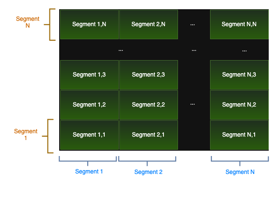
To support compound keys, we needed to define a search space that would allow for all the key types (integers, alphanumerics, and UUIDs) to intermingle, and be easy to segment, ideally using as few WHERE expressions as possible. Our solution was to treat the compound key as a vector space with N dimensions, where N is the number of columns in the key. That allows for segmenting each column separately, on its own "dimension", and using these points to divide the space into N-dimensional segments, creating a grid-like structure.
With these segmentation techniques in place, we now have all the building blocks needed to implement our diffing algorithm. The next section will explore how we put these pieces together to implement the algorithm.
Part 3 - Implementing the diff
By now, we have both a consistent cross-database hashing function, and an efficient way to split the table, the two key abstractions that we need in order to implement our divide-and-conquer diff algorithm. We already introduced the algorithm, but let's have another look.
Our diff follows the following steps:
- Split both tables into corresponding segments based on their primary keys
- Calculate a hash checksum for each segment pair
- Compare the hashes:
- If the hashes match → The segments are identical.
- If the hashes differ → We have two options:
- For small segments: Download both segments and compare them in memory
- For large segments: Recursively split them into smaller pieces and repeat the process
Reladiff's implementation follows this exact logic, but also:
- Runs in parallel - Each comparison enters a task queue with a priority based on search depth. "Recursion" happens through this queue.
- Yields early - With depth-first prioritization, we produce initial results quickly and can potentially terminate early.
- Is conservative - When users cap maximum results, the algorithm stops as soon as the limit is reached.
- Analyzes the table schema to ensure normalized value comparisons (more on this later).
The performance profile of this algorithm ranges from O(n) when all data is identical, up to O(n²) when all data differs. In a situation when the data is mostly different, and the differences are spread out, it would be better to skip the hashing and just download all the data directly. But for our intended use-cases, which are mainly validation and testing incremental change, we can expect good performance on average.
Bisection factor & threshold
The two major parameters of the diffing algorithm are the bisection factor, which determines how many segments to split into each time, and the bisection threshold, which determines when a segment is small enough to download, instead of bisecting it.
The bisection factor in Reladiff, by default, is 32. We found it to be a good balance for the common use-case, as it allows us to take advantage of a high thread-count, while not creating too many segments, which could flood the database with too many separate queries, and hurt performance. In very large tables, a higher bisection factor might be needed, to avoid time-outs or even sum overflows. We leave this choice in the hands of the user, because counting the table before we start, would delay the diff by too much. But perhaps an optional auto-tuning of the bisection factor could be a nice feature.
The bisection threshold in Reladiff is 16K rows by default. This means that tables or segments with fewer than 16K rows will be downloaded, instead of bisected. Here too, we found it to strike a good balance, based on empirical testing. However, users might wish to adjust it based on their network speed. Slow networks might benefit from a lower threshold, and fast networks from a much higher one. Increasing it can also lighten the computational burden on the database, at the cost of increased I/O.
Multi-threading
Most classical databases, such as PostgreSQL and MySQL, execute each query in its own single thread. The only way to parallelize the query (bar plugins), is by making multiple smaller queries. Notable exceptions are the cloud databases, such as Snowflake or BigQuery, which are able to parallelize their execution on their own. But for the majority of databases that can't, table splitting can speed up a wide variety of algorithms, just by the nature of running them in parallel. Amusingly enough, it can even speed up a SELECT COUNT(*) query by a big factor. But while it reduces the waiting time, it may also put a sudden load on the database. So while very useful, heavy parallelization should be used mindfully.
Duplicate rows
When diffing on tables that don't constrain their primary key, or don't have one, we are faced with the possibility of duplicate rows. Fortunately, duplicates don't interfere with our divide-and-conquer mechanism at all. To support them, we only have to make sure our diffing operation counts the unique items in each table, and subtract the corresponding counts from each other. However, in the extreme case of thousands of duplicates, it might skew the table distribution enough to affect the speed of the diff.
Schema negotiations
We query the schema of both tables before we begin the diff, for three reasons. First, we want to know the types of each column, so we can validate that the types can be compared, and that the key column types can be used for keyset segmentation. Secondly, we want to find out the precision of each column, so that we can normalize the values correctly, using the smallest available precision. The third reason is to detect whether text columns are alphanumeric or UUID.
See, alphanumeric columns are just regular text columns (of type CHAR or VARCHAR), that happen to only contain alphanumeric values. The only way for us to know if they are alphanumeric or not, is to sample a few values, and check if they are all alphanumeric, under the assumption that a non-alphanumeric column is unlikely to conform by accident. We can support alphanumerics because their lexicographic order is predictable and consistent across all the databases we support, with the surprising exception of MySQL. However, ordering arbitrary text is not consistent, and it produces different results on different databases. So once we detect in the schema that a column is text, we sample it, and if its values are all alphanumerics, or all UUIDs, we treat them accordingly. (while PostgreSQL has a native UUID type, most databases don't)
Fortunately, most databases support the same SQL-based interface for querying the schema, although there are small but significant differences. Different databases have different names for their data-types, different ways of specifying precision, and a different way of doing namespaces, if they do them at all. A few of the databases, for example Databricks, use their own unique interface.
Example SQL query to extract the column information we need, that works for most of the databases we support:
SELECT column_name, data_type, datetime_precision, numeric_precision, numeric_scale
  FROM information_schema.columns
  WHERE table_name = '{name}' AND table_schema = '{schema}'
Eager diffing (or: hit the ground running)
The first step for segmentation is to query the min/max values for every column across both tables. By merging these key ranges for each column pair, we ensure all the rows from both tables fall within our segmentation. But here lies an opportunity for optimization. These queries often go to two different databases, and that means one can return a lot sooner than the other. For one thing, the min/max values of a column are sometimes cached, and return instantly, and sometimes they are not, and can take many seconds to return. It's usually cached in local databases such as PostgreSQL, and isn't cached in cloud databases such as Snowflake. Other possible causes for a late response include network latency, server warmup, or high server load. Waiting for responses from both databases would unnecessarily delay the beginning of the diffing process, and the time to first response.
Luckily, we can avoid waiting. We can start diffing the first range we get, and when the second range arrives, diff whatever segments we missed, if any. So, for example, if the first range is [1, 10], we can start diffing within those values, and when the second range arrives, say [5, 15], we can diff between the values of [10, 15].
Below is a visualization comparing one-dimensional and two-dimensional compound keys. In both of them, table 2 returns its key range first, which allows the diff to begin on the known subset, marked by pass #1. Later the key range of table 1 returns, which allows us to diff the remaining subsets in pass #2.
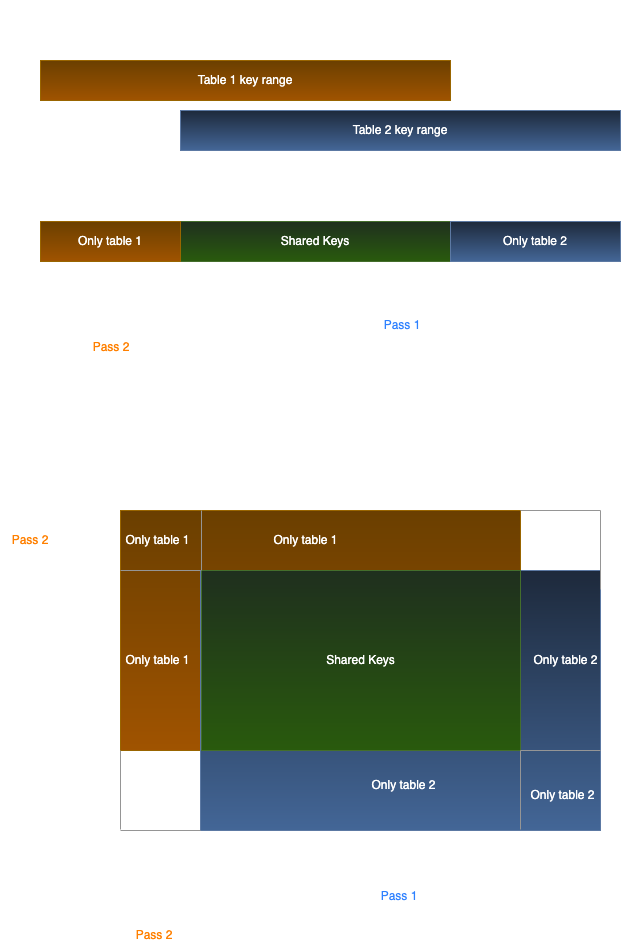
In our example, both the 1D and 2D tables have exclusive values to each other, but we should be ready for all possible situations. For example, one table may contain the other completely, and we may begin either with the containing table, or with the contained table.
Worth noting that in the 1D version, the second pass may include up to 2 new regions, if the first key-range is enveloped by the second key-range. In the 2D version, it may include 8 new regions (imagine a tic-tac-toe board, where we only marked the center). To generalize, the max number of new regions in the 2nd pass is (3^k)-1, where k is the number of dimensions.
Use JOIN when possible
When the tables we want to diff reside in the same database, we can just use an OUTER JOIN, which should always be faster than using hashes and bisection. An OUTER JOIN guarantees to include all the rows from both tables, but it will also remove duplicate rows, and even rows that have different data, but duplicate keys. When diffing rows whose keys are not unique, it's still better to use the hash-diff.
The work we've done on splitting the table will still serve us well here too. Running a join on a very large table can easily time-out. Moreover, we can make the join a lot faster if we run it in parallel. For both of these reasons, we bisect the table, once, before running the OUTER JOIN on each of the pairs of segments.
Conclusion
Reladiff's journey to become production-ready was long and challenging. We navigated a long list of limitations in SQL, some anticipated but some very unexpected. But with a combination of creative solutions and attention to detail, and a few unfortunate compromises, we were able to deliver convincing results. The significant performance gains we achieved over conventional approaches give optimism for improvements in the data-engineering ecosystem.
Table segmentation emerges as a very performant technique, that can improve the performance of many database tools. For any task, ranging from counting a table, to making analytical queries, or large joins, the response time of the tool can be significantly improved with segmentation, and with it, the user experience.
We might also imagine diff-powered tools for live cross-database synchronization, or services for lightweight incremental backups.
And yet, implementing these techniques can at times be complicated, and there are many details to consider, as we've shown above. However, most of our complications came from the need to be consistent across databases. It's much easier when only one table is involved. For Python, at least, Sqeleton contains most of the infrastructure code for implementing keyset segmentation, and the remaining parts can be easily adapted from Reladiff. But at the moment, there isn't yet a user-ready API that takes care of all the details.
I remain optimistic about the future of database tooling, but I recognize the path forward isn't easy. Only determined engineers, with a good understanding of user needs, will be able to pierce through.
If you would like to know more about Reladiff, you can:
- check out the documentation: https://reladiff.readthedocs.io/en/latest/
- or visit the project repo on GitHub: https://github.com/erezsh/reladiff
If you're in need of an expert consultant, contact us! We are currently accepting new clients.